Introduction
If you feel like experimenting yourself, the NT hash dataset can be generated using this creatively-named script.
In Part 1 we retrieved NTDS and in Part 2 we organised it using hash-organiser. We are now ready to move to the next part of the process: recovering hashes.
Extract NTDS → Clean/Organise NTDS → Crack hashes → Generate stats.
“Cracking hashes” sounds a bit abstract, so let’s try narrowing it down. At this stage, the goal is not to crack as many hashes as possible just because, but to identify weak passwords and patterns that represent real risk to the domain.
First, let’s remind ourselves some potential limitations we might have, so we can agree what is out of scope:
- Password auditing is just one part of an internal assessment, therefore, we can only allocate a limited amount of time to it. Creating OSINT-based custom wordlists is not an option here. Although there are some interesting tools out there, to keep things simple, we will opt for using generic wordlists for now.
- Our weapon is an average-performance work laptop which we might have to use for other tasks in parallel with cracking. Thus, there is a good chance that we can’t even dedicate the laptop’s full resources to cracking.

Let’s start by talking about some terminology before diving into the practical aspect.
Hash Rate, Keyspace, and Cracking Time
Before we start cracking on terminology (pun intended!), we need to make sure that we are running hashcat on our native host utilising our GPU. The oversimplified reasoning for this is that more layers lead to more overhead which lead to less efficiency. If you are not convinced, have a look at the numbers below (Windows+GPU vs. WSL2+CPU):
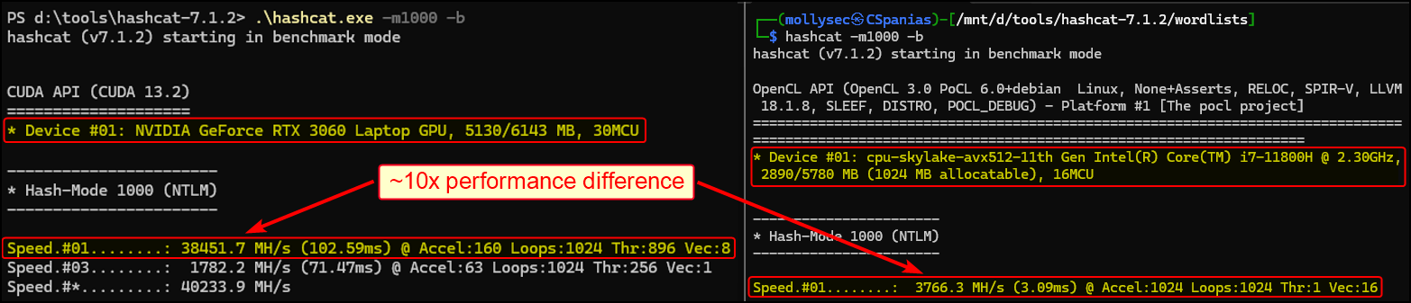
The number highlighted above is the hash rate which translates to hash calculations per second. In our case:
- 1 Megahash per second (MH/s) = 1,000,000 Hashes per second (H/s)
- 38,451.7 MH/s x 1,000,000 = 38,451,700,000 H/s
It is worth mentioning that the hash rate obtained through benchmarking (-b) measures only raw hashing, i.e., with the GPU 100% dedicated to hashing. Actual cracking involves generating candidates (reading wordlists, applying rules, handling rejections, etc.), which introduces significant overhead.
In practice, the GPU spends part of its time waiting for new candidates instead of hashing continuously, so the effective speed drops significantly. For example, in our case, there is a ~5x difference between the benchmark speed (~38,452 MH/s) and the actual hash rate (~7,969 MH/s) as we will soon see!
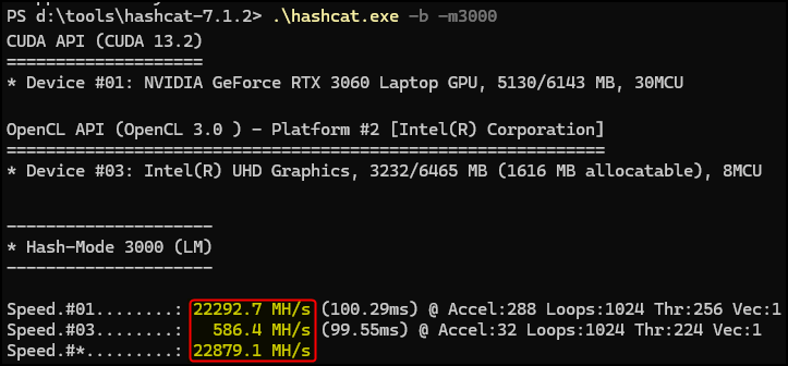
Although we are interested mostly in NT hashes here, it is good to know that the hash rate is also affected by the format of the hash. For example, LM hashes are considerably weaker (easier to crack) than NT hashes, but the hash rate (on my setup) for LM is ~1.8x lower than that of NT (~23k MH/s vs. ~38k MH/s). This is due to the way LM hashing works internally, which makes it less GPU-friendly:
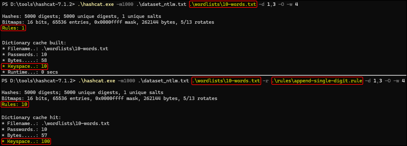
The next term we care about is the keyspace, the total number of possible guesses. For instance:
- A run using a 10-word wordlist would only have to try these 10 words. Thus, the keyspace would be 10.
- Adding a 10-rule ruleset would increase the keyspace to 10 x 10 = 100 (10 rules applied to every password).
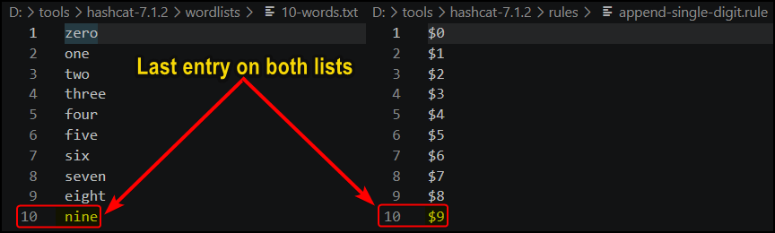
Dividing the keyspace by the hash rate give us the estimated cracking time. This represents the worst-case scenario, where every possible candidate must be tested. It assumes that either no hashes are recovered, or that any recovered hashes only appear at the very end of the candidate space (i.e. the last entry in the wordlist and/or the last rule applied).
For example, the estimated cracking time using the above 10-word wordlist and 10-rule ruleset combination would assume that either no hashes will be recovered or every recovered hash will result to nine9, forcing an iteration of all possible candiates for every hash:
zero0,zero1, …,zero8,zero9(10 total candidates)one0, …,nine9(90 total candidates)nine0,nine1, …,nine8,nine9(100 total candidates)
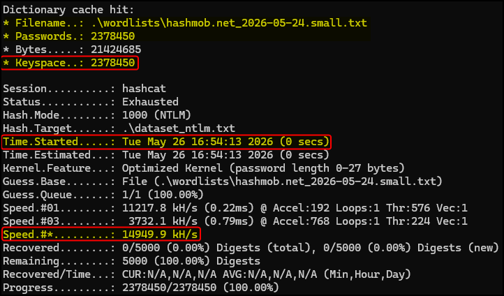
Let’s estimate the cracking time for a more realistic example using the small hashmob wordlist at 14,949.9 kH/s:
- The wordlist contains 2,378,450 passwords which represents the keyspace.
- The hash rate is 14,949.9 kH/s × 1000 = 14,949,900 H/s.
- The estimated cracking time is 2,378,450 / 14,949,900 = ~0.16 milliseconds (ms).
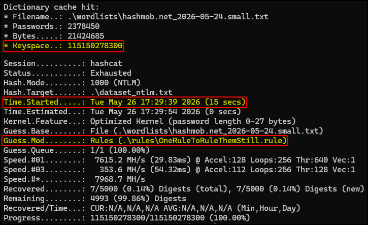
As expected, the bigger the keyspace, the more time we will need to spend on cracking. For instance, if we throw some rules to the mix, the keyspace will increase from ~2,4 million to 115+ billion guesses(!):
- Keyspace: 2,378,450 (wordlist) × 48,439 (rules) = 115,150,278,300
- Hash rate: 7,968.7 MH/s x 1,000,000 = 7,968,700,000 H/s
- Cracking time: 115,150,278,300 / 7,968,700,000 = ~14.5 secs
Now we are done with the theory, let’s see how all these work in practice.
Cracking Methodology
Go Simple, Go Big
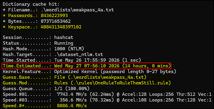
The simplest way to crack our hashes is to grab a large wordlist along with a good ruleset and just let it run. The combination below has a keyspace of 408+ trillion guesses and an estimated time of 14 hours:
This approach requires minimal effort and it could be fitting if the plan is to leave the laptop working during out-of-work hours. When the run is done, we move directly to the next step by passing the potfile to our analysis tool.

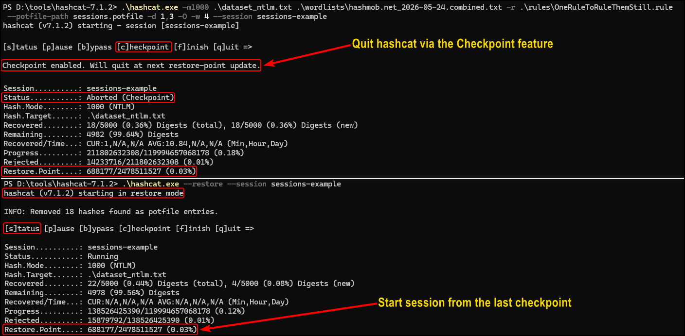
In this case, we can utilise hashcat sessions by leaving hashcat running overnight, create a checkpoint right before we need the laptop in the morning, and then resume the session when we no longer need it for the day:
One downside of this method is the assumption that all hashes are of equal strength. What if there are some extremely weak passwords that could be recovered with just a small wordlist and no rules at all in just a few seconds?
Start Small, Go (Progressively) Big
At first glance, this approach looks pretty straightforward, but I totally got the wrong idea when I first saw it.

In my ignorant brain, this seemed as a smart approach because, for some unknown reason, I thought that by reducing the pool of hashes passed to the final run would somehow make it faster.

Let’s see how dumb I was in practice. Below are four runs, each one more expensive than the previous:
| Run | Wordlist Size | Keyspace (~) | Cracked Hashes | Total Cracked Hashes | Duration (hh:mm:ss) |
|---|---|---|---|---|---|
| 1 | Small | 115 Billion | 7 | 7 | 00:00:15 |
| 2 | Medium | 709 Billion | 31 | 38 | 00:01:31 |
| 3 | Large | 3 Trillion | 242 | 280 | 00:06:30 |
| 4 | Huge | 120 Trillion | 1,260 | 1,540 | 04:16:00 |
| Total | - | - | 1,540 | - | 04:24:16 |
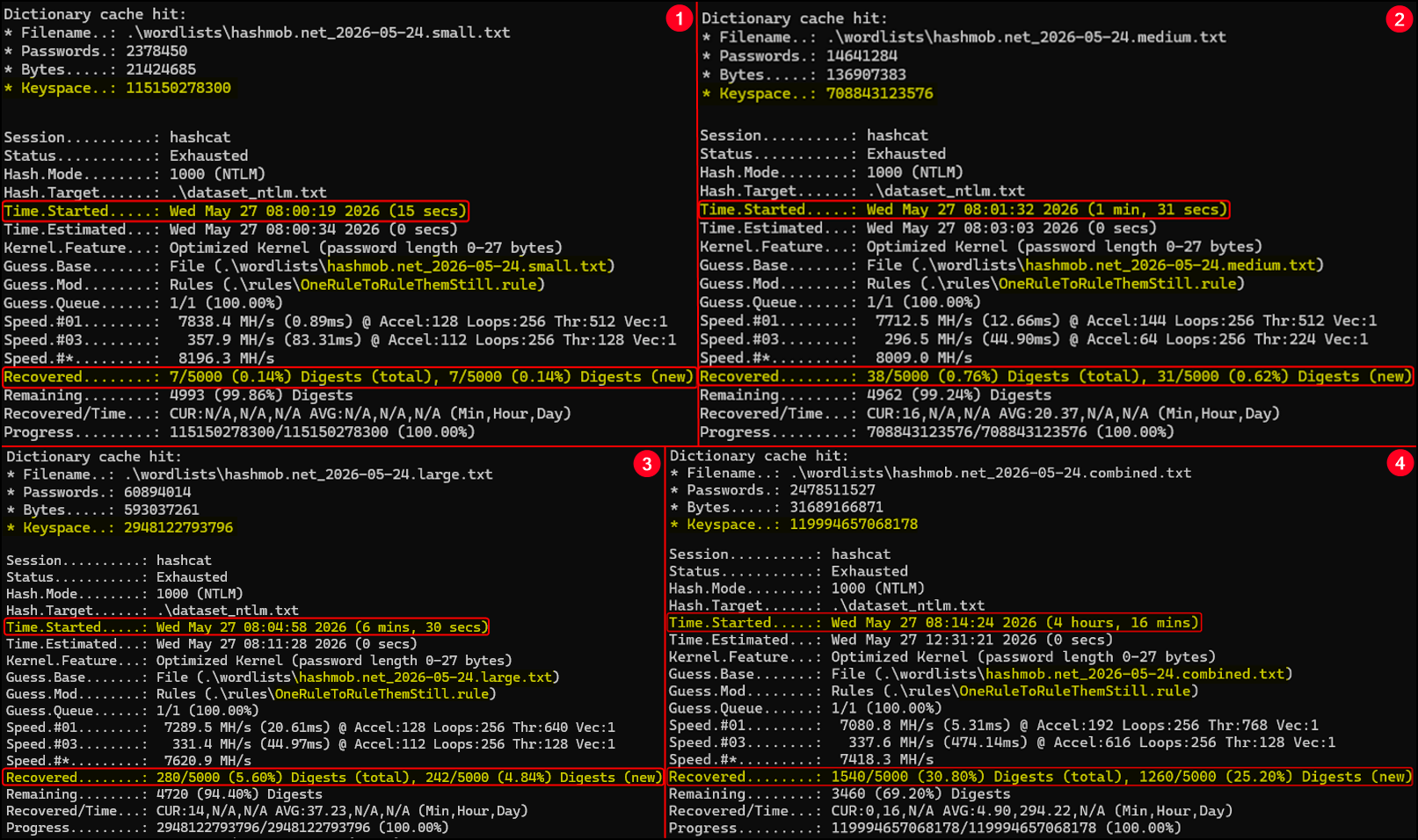
We managed to recover a total of 280 hashes during the first three runs, so we reduced the pool from 5k down to 4,720 hashes. So the 4th run should be faster now, right?
To validate my ignorance, let’s check what the numbers would be if I instead had run just the 4th run right away:
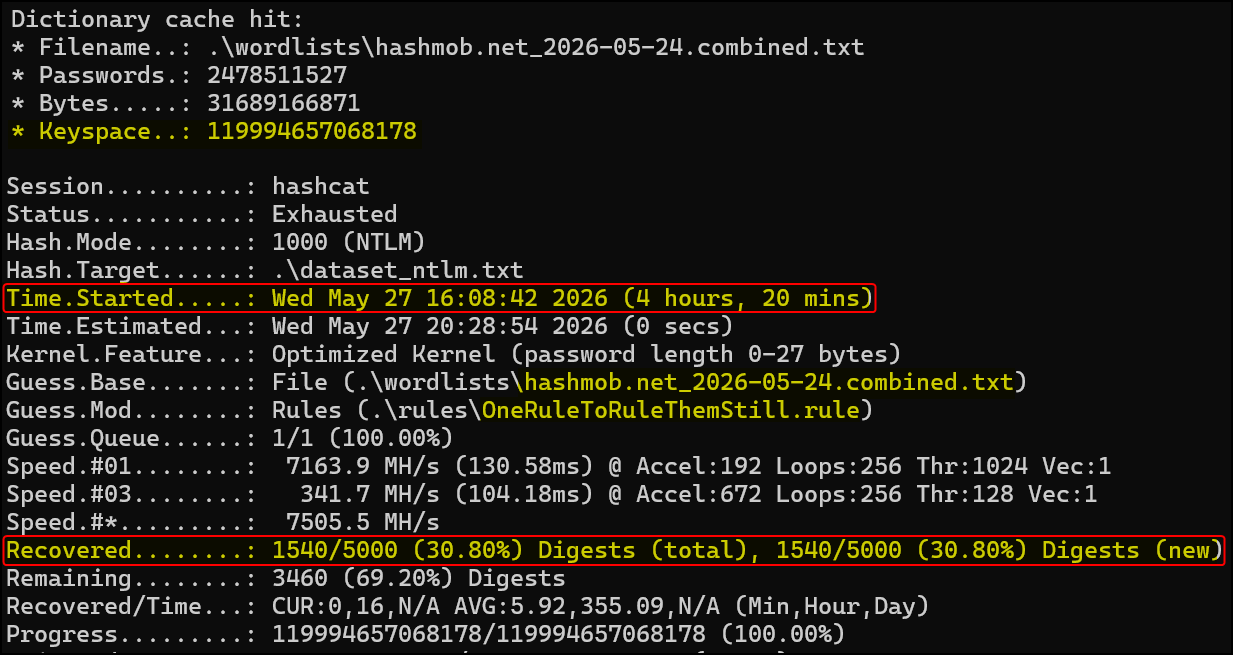
Almost no difference! However, if you know what you are doing (unlike me), that’s not really a surprise, but actually expected since cracking time is mostly driven by the size of the keyspace rather than the number of target hashes.
In this case, since we used the exact same wordlist and ruleset, we ended up with the exact same keyspace: ~120 trillion guesses. Although a larger number of hashes increases comparison overhead, this cost is minor compared to the expense of generating and testing candidates, making its impact on overall runtime relatively small.
From a time-optimisation perspective, the only benefit of the phased approach I could think of is when working towards a cap. For instance, if our goal is to crack x% of hashes as a PoC, we could try to achieve that before reaching the 4th step, i.e., completely avoiding running the expensive step altogether.
But is there more to it than just runtime optimisation?
Optimising the Dataset’s Value
So you might be wondering, why the puck am I reading this?
While this approach does not optimise runtime, it changes what we can learn from the cracking process.
Think of it not from a time-optimisation but from information-optimisation perspective. If we stick to the first approach (Go Simple Go Big), we will get a single potfile showing that we recovered 30.8% of the hashes.
But why not squeeze some more information from this step of the process?
By running attacks in stages we could extract insights about user behaviour. For example, we could map each phase to approximate password strength categories based on the effort required to crack them:
| Phase | Recovered Hashes | Password Strength | Remediation Priority |
|---|---|---|---|
| 1,2 | 38 | Extremely Weak | Highest |
| 3 | 242 | Weak | High |
| 4 | 1,260 | Medium | Medium |
Generating stats based on the cracked hashes is the topic of Part 4, so I am not talking about that here. When we are on a client debrief and discussing the password audit phase, I have found an increased client engagement in presenting the results in a more “interesting” way rather than just showing them boiler-plate statistics.
Which statement do you think has more chances to obtain buy-in from the client:
We cracked 30% of the domain hashes.
or:
Six percent of the domain users are using extremely weak passwords that are vulnerable to low-effort attacks.
In my opinion, the latter has more chances to make the client engaged in the conversation resulting in follow-up questions. This makes the discussion more interesting, makes me more motivated, and the client has a higher chance to come back, which makes the company I work for happier as well! A classic win-win-win situation.

Now that we have an idea of what we want, let’s jump to everyone’s favourite pastime: vibe-coding!
Vibe-Coding
The main idea here is similar to our previous PoC: vibe-code a minimal PoC for automating the above process. We used Bash to create hash-organiser, so, for a breath of fresh air, this time we will use Python.

For this PoC, instead of producing an all encompassing script, I decided to have a JSON file that the script will have to parse. The main reasons for this choice were:
- I didn’t want to lose any native
hashcatfunctionality (I wanted to have the ability to use all of its flags). - I wanted to be able to configure and test different phases relatively easy.
- I wanted to have “templates” that could be handy for audit purposes (i.e., identical workflows) as well as for different cracking contexts (e.g. different timelines).
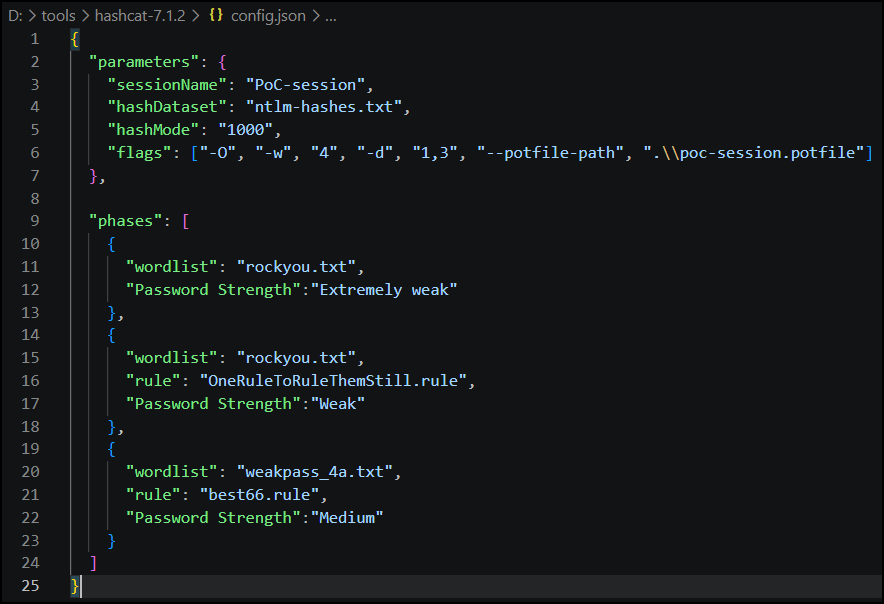
Let’s get to the point. Within this JSON file there are two root keys:
- The
parameterskey takes thehashcat-related stuff (e.g. hash file, hash mode, potfile, etc.). - The
phaseskey contains the phase-related details (e.g. wordlist and ruleset).
Any additional key-value pair passed to
phases, is added as a column on the final table (--report).
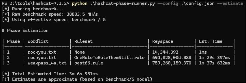
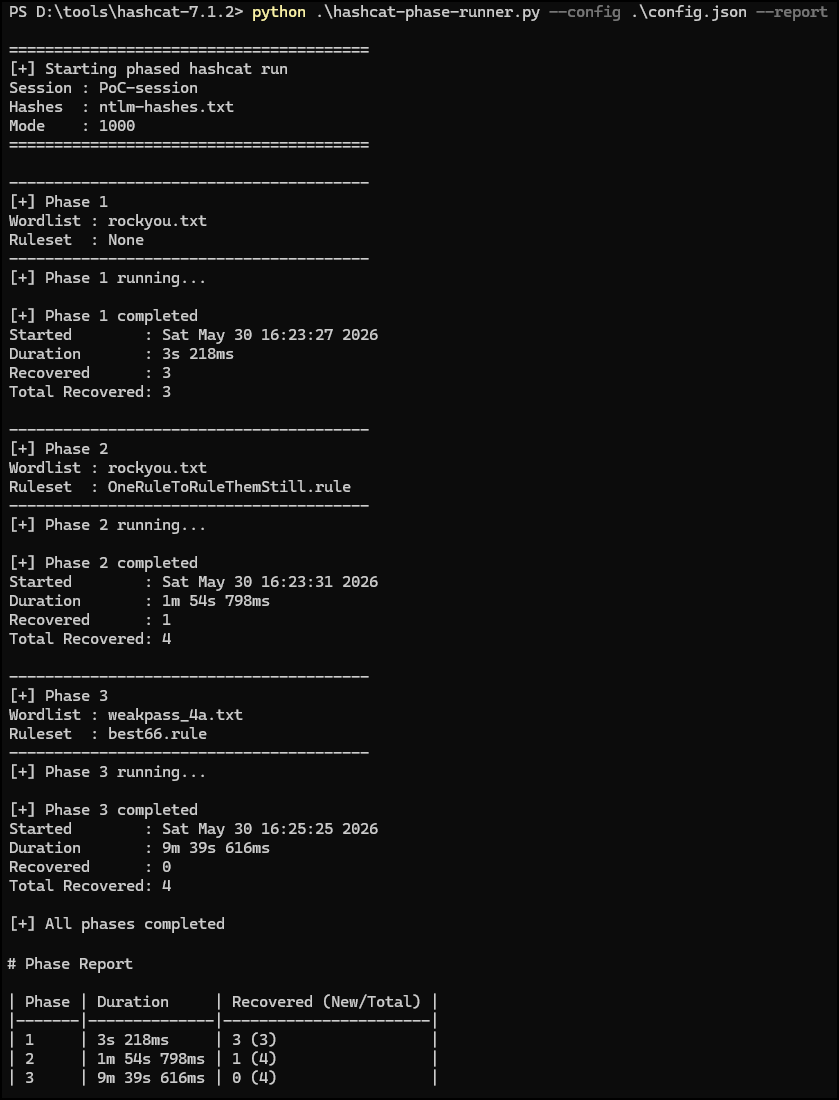
The mighty phase-cracker PoC has two main functions. Either it calculates the keyspace of each phase and provides a wildly-off estimated cracking time (--estimate) or it just executes all configured runs (--estimate flag omitted):
Conclusion
Cracking passwords is often seen as a purely technical task, with the goal of optimising runtime and increasing the percentage of cracked hashes. However, the way we approach cracking can significantly affect the value we extract from it, allowing us to move beyond a simple “cracked vs. not cracked” metric.
In the next (and final) part, we will look at ways to analyse hashcat’s potfile and extract (hopefully) meaningful statistics.

Next: [Password Audits Part 4: Analysing Results →]